Scientific Computing in Python

This is a sample of doing some real scientific computing in Python.

We refer to some ideas in the book "Python for Scientists" by John M. Stewart. Specifically, we want to explore a numerical solver for ordinary differential equations (ODEs), called ODEint. This solver is based on lsoda, a Fortran package from Lawrence Livermore Labs that is a reliable workhorse for solving these difficult problems.

We look at four different ODEs that are interesting, and numerically challenging. They are:

the harmonic oscillator (or linear pendulum)
the non-linear pendulum
the Lorenz equation, which is the model for chaotic behaviour
the van der Pols equation, which is an example of a stiff ODE with periodic behaviour.

We do some basic tests of an ODE numerical solver, to test its accuracy, and to consider whether our asymptotic analysis of a pendulum is any good.

As in previous examples, we must start with code to tell the Notebook to plot items inline, and load in packages to do numerical computations (numpy), scientific computation (scipy) and plotting (matplotlib).

%matplotlib inline
import numpy as np
import matplotlib.pyplot as plt
from scipy.integrate import odeint # This is the numerical solver

We start with a second order linear equation, that has the usual harmonic oscillator solutions.

$y''(t) + \omega^2 y(t) = 0, \qquad y(0) = 1, y'(0) = 0.$

To put this into the numerical solver, we need to reformulate as a 2 dimensional, first order system:
$\mathbf{y} = (y,y')^T, \qquad \mathbf{y}'(t) = (y', -\omega^2 y)^T.$
Here is a simple code snippet that solves the problem numerically.

def rhs(Y,t,omega):  # this is the function of the right hand side of the ODE
    y,ydot = Y
    return ydot,-omega*omega*y

t_arr=np.linspace(0,2*np.pi,101)
y_init =[1,0]
omega = 2.0
y_arr=odeint(rhs,y_init,t_arr, args=(omega,))
y,ydot = y_arr[:,0],y_arr[:,1]
plt.ion()
plt.plot(t_arr,y,t_arr,ydot)

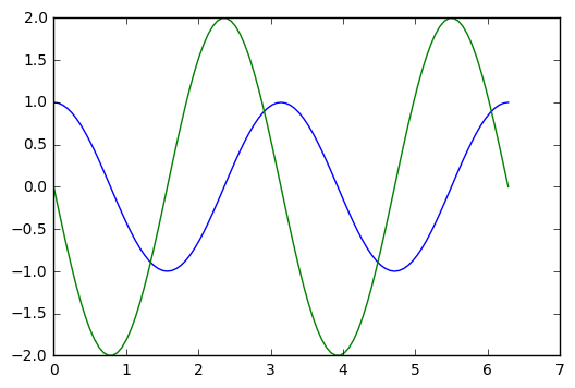
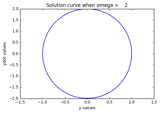
# Let's draw a phase portrait, plotting y and ydot together
plt.plot(y,ydot)
plt.title("Solution curve when omega = %4g" % omega)
plt.xlabel("y values")
plt.ylabel("ydot values")

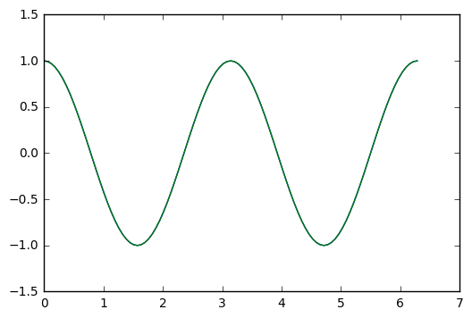
Now, I would like to test how accurate this numerical code is, by comparing the exact solution with the numerical solution. The exact solution is given by the initial values of y_init, and omega, and involves cosines and sines.

t_arr=np.linspace(0,2*np.pi,101)
y_init =[1,0]
omega = 2.0
y_exact = y_init[0]*np.cos(omega*t_arr) + y_init[1]*np.sin(omega*t_arr)/omega
ydot_exact = -omega*y_init[0]*np.sin(omega*t_arr) + y_init[1]*np.cos(omega*t_arr)
y_arr=odeint(rhs,y_init,t_arr, args=(omega,))
y,ydot = y_arr[:,0],y_arr[:,1]
plt.plot(t_arr,y,t_arr,y_exact)

# We plot the difference
plt.plot(t_arr,y-y_exact)

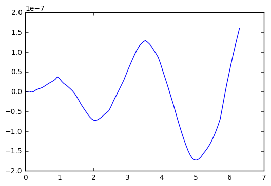
So, in the test I did above, we see an error that oscillates and grows with time, getting to about size 2x 10^(-7). Which is single precision accuray.

Now, apparently ODEint figures out good step sizes on its own. Let's try running the code again, with different number of steps in the t-variable.

numsteps=1000001  # adjust this parameter
y_init =[1,0]
omega = 2.0
t_arr=np.linspace(0,2*np.pi,numsteps)
y_exact = y_init[0]*np.cos(omega*t_arr) + y_init[1]*np.sin(omega*t_arr)/omega
ydot_exact = -omega*y_init[0]*np.sin(omega*t_arr) + y_init[1]*np.cos(omega*t_arr)
y_arr=odeint(rhs,y_init,t_arr, args=(omega,))
y,ydot = y_arr[:,0],y_arr[:,1]
plt.plot(t_arr,y-y_exact)

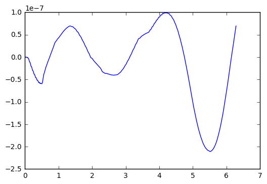
Okay, I went up to one million steps, and the error only reduced to about 1.0x10^(-7). Not much of an improvement.

Let's try another experiment, where we go for a really long time. Say 100 time longer than the example above.

numsteps=100001  # adjust this parameter
y_init =[1,0]
omega = 2.0
t_arr=np.linspace(0,2*1000*np.pi,numsteps)
y_exact = y_init[0]*np.cos(omega*t_arr) + y_init[1]*np.sin(omega*t_arr)/omega
ydot_exact = -omega*y_init[0]*np.sin(omega*t_arr) + y_init[1]*np.cos(omega*t_arr)
y_arr=odeint(rhs,y_init,t_arr, args=(omega,))
y,ydot = y_arr[:,0],y_arr[:,1]
plt.plot(t_arr,y-y_exact)

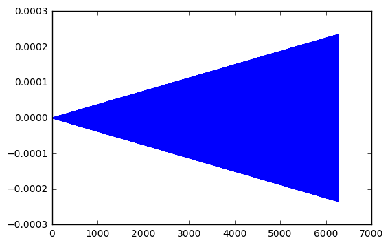
Interesting. My little test show the error grow linearly with the length of time. In the first time, 2x10^(-7). For 10 times longer, 2x10^(-6). For 100 times longer, 2x10^(-5). And so one.

A more subtle question: are these amplitude errors, or phase errors, or perhaps a combination?

p1=np.size(t_arr)-1
p0=p1-100
plt.plot(t_arr[p0:p1],y[p0:p1],t_arr[p0:p1],y_exact[p0:p1])

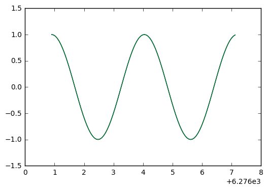
plt.plot(t_arr[p0:p1],y[p0:p1]-y_exact[p0:p1])

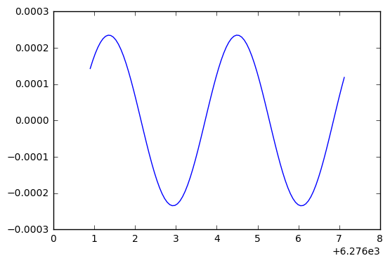
Ah ha! This looks like the negative derivative of the solution, which indicates we have a phase error. Because with phase error, we see the difference
$\cos(t + \delta) - \cos(t) \approx -\delta\cdot \sin(t)$
while with an amplitude error, we would see
$(1+\delta)\cos(t) - \cos(t) \approx \delta\cdot \cos(t).$

Let's plot the soluton and the error difference, to see if the derivative zeros line up with peaks.

plt.plot(t_arr[p0:p1],y_exact[p0:p1],t_arr[p0:p1],3000*(y[p0:p1]-y_exact[p0:p1]))

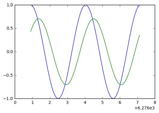
Looking at the above, we see they don't quite line up. So a bit of phase error, a bit of amplitude error.

The non-linear pendulum

Well, it's not to hard to generalize this stuff to the non-linear pendulum, where the restoring force has a sin(t) in it. We want to observe the period changes with the initial conditions (a bigger swing has a longer period).

The differential equation is:

$y''(t) + \omega^2 \sin(y(t)) = 0, \qquad y(0) = \epsilon, y'(0) = 0.$

To put this into the numerical solver, we need to reformulate as a 2 dimensional, first order system:

$\mathbf{y} = (y,y')^T, \qquad \mathbf{y}'(t) = (y', -\omega^2 \sin(y))^T.$

Here is a simple code snippet that solves the problem numerically.

def rhsSIN(Y,t,omega):  # this is the function of the right hand side of the ODE
    y,ydot = Y
    return ydot,-omega*omega*np.sin(y)

omega = .1   # basic frequency
epsilon = .5 # initial displacement, in radians (try 0 to .5)
velocity = 0 # try values from 0 to .2
t_arr=np.linspace(0,2*100*np.pi,1001)
y_init =[epsilon,velocity]

# we first set up the exact solution for the linear oscillator
y_exact = y_init[0]*np.cos(omega*t_arr) + y_init[1]*np.sin(omega*t_arr)/omega
ydot_exact = -omega*y_init[0]*np.sin(omega*t_arr) + y_init[1]*np.cos(omega*t_arr)
y_arr=odeint(rhsSIN,y_init,t_arr, args=(omega,))
y,ydot = y_arr[:,0],y_arr[:,1]
plt.ion()
plt.plot(t_arr,y,t_arr,y_exact)

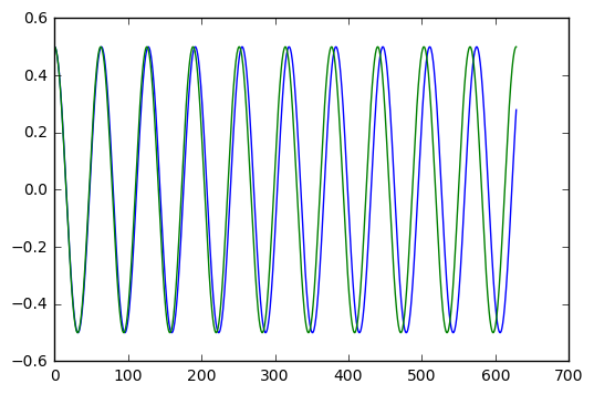
With epsilon = 0.1 (radians, which is about 5.7 degrees), it is hard to see a period shift. With epsilon = 0.5 (radians, which just under 30 degrees), we clearly see a shift after ten cycles of oscillation.

How big is the shift? Can we figure this out easily with numerics? And how does it compare with the estimate given by the Poincare-Lindstedt method?

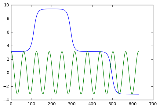
It is kind of fun to set this up with epsilon = pi, which corresponds to an inverted pendulum. The pendulum sits upside down for a while, then slowly moves away from this unstable equilibrium point. The behaviour is very different than the linear harmonic oscillator. We show the example in the next cell.

omega = .1   # basic frequency
epsilon = np.pi+.0001 # initial displacement, in radians (try 0 to .5)
velocity = 0 # try values from 0 to .2
t_arr=np.linspace(0,2*100*np.pi,1001)
y_init =[epsilon,velocity]

# we first set up the exact solution for the linear oscillator
y_exact = y_init[0]*np.cos(omega*t_arr) + y_init[1]*np.sin(omega*t_arr)/omega
ydot_exact = -omega*y_init[0]*np.sin(omega*t_arr) + y_init[1]*np.cos(omega*t_arr)
y_arr=odeint(rhsSIN,y_init,t_arr, args=(omega,))
y,ydot = y_arr[:,0],y_arr[:,1]
plt.ion()
plt.plot(t_arr,y,t_arr,y_exact)

The Lorenz equation

You've probably heard of the butterfly effect (it's even a movie). The idea is that weather can demonstrate chaotic behaviour, so that the flap of a butterfly wing in Brazil could eventually result in a tornado in Alabama.

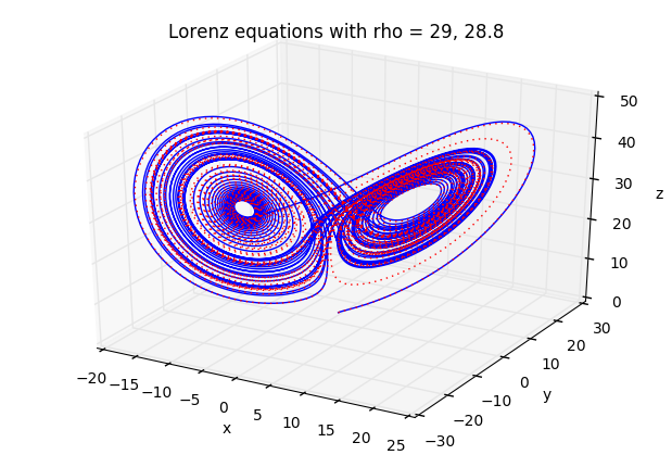
Lorenz was studying a simplified model for weather, given by a system of three simple ODEs:

$x' = \sigma(y-x), \quad y'=\rho x - y - xz, \quad z' = xy - \beta z$

where $x,y,z$ are functions of time, and $\sigma, \rho,\beta$ are fixed constants.

When $\rho$ is small, the behaviour is quite predictable. But when $\rho$ gets better than about 24.7, you get strange, aperiodic behaviour.

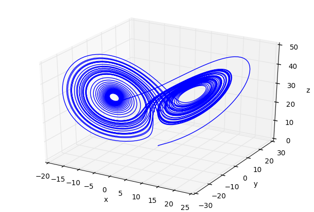
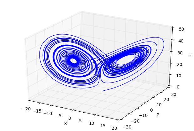
Here is some code that demonstrates the behaviour. We also include 3D plots

def rhsLZ(u,t,beta,rho,sigma):
    x,y,z = u
    return [sigma*(y-x), rho*x-y-x*z, x*y-beta*z]

sigma = 10.0
beta = 8.0/3.0
rho1 = 29.0
rho2 = 28.8  # two close values for rho give two very different curves

u01=[1.0,1.0,1.0]
u02=[1.0,1.0,1.0]

t=np.linspace(0.0,50.0,10001)
u1=odeint(rhsLZ,u01,t,args=(beta,rho1,sigma))
u2=odeint(rhsLZ,u02,t,args=(beta,rho2,sigma))

x1,y1,z1=u1[:,0],u1[:,1],u1[:,2]
x2,y2,z2=u2[:,0],u2[:,1],u2[:,2]

from mpl_toolkits.mplot3d import Axes3D

plt.ion()
fig=plt.figure()
ax=Axes3D(fig)
ax.plot(x1,y1,z1,'b-')
ax.plot(x2,y2,z2,'r:')
ax.set_xlabel('x')
ax.set_ylabel('y')
ax.set_zlabel('z')
ax.set_title('Lorenz equations with rho = %g, %g' % (rho1,rho2))

fig=plt.figure()
ax=Axes3D(fig)
ax.plot(x1,y1,z1)
ax.set_xlabel('x')
ax.set_ylabel('y')
ax.set_zlabel('z')

fig=plt.figure()
ax=Axes3D(fig)
ax.plot(x2,y2,z2)
ax.set_xlabel('x')
ax.set_ylabel('y')
ax.set_zlabel('z')

You should play around with the time interval (in the definition of varible t) to observe the predictable, followed by chaotic behaviour. ANd play with other parameters.

van der Pol equation

This equation is used as a testbed for numerical software. It is nonlinear, and collapses to a periodic orbit very quickly. We can include information about the Jacobian, the derivative of the vector function $\mathbf{f}$
in the ODE system $\mathbf{y}' = \mathbf{f}(\mathbf{y},t)$ , into the ODE solver, to help it choose appropriate step sizes and reduce errors.

The van der Pol equation is this:

$y'' - \mu(1-y^2)y' + y = 0$

with the usual initial conditons for $y(0), y'(0)$ . In vector form, we write

$\mathbf{y} = (y,y')^T, \qquad \mathbf{f}(\mathbf{y}) = (y', \mu(1-y^2)y' - y)^T.$

The Jacobian is a 2x2 matrix of partial derivatives for $\mathbf{f}$ , which is

$\mathbf{J}$\mathbf{y}$ = \left$ \begin{array}{cc} 0 & 1 \ -2\mu y \* y' -1 & \mu\(1-y^2$ \end{array} \right\)$

We set up the code as follows:

def rhsVDP(y,t,mu):
    return [ y[1], mu*(1-y[0]**2)*y[1] - y[0]]

def jac(y,t,mu):
    return [ [0,1], [-2*mu*y[0]*y[1]-1, mu*(1-y[0]**2)]]

mu=3 # adjust from 0 to 10, say
t=np.linspace(0,30,10001)
y0=np.array([2.0,0.0])
y,info=odeint(rhsVDP,y0,t,args=(mu,),Dfun=jac,full_output=True)

print("mu = %g, number of Jacobian calls is %d" % (mu, info['nje'][-1]))

plt.plot(t,y)

mu = 3, number of Jacobian calls is 0

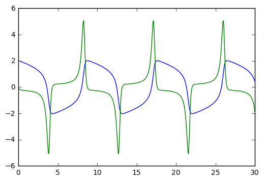
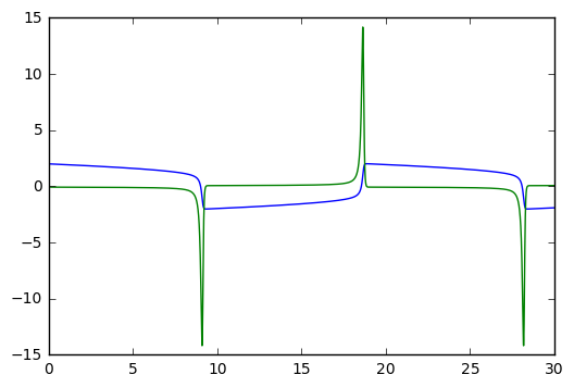
Try playing with the mu parameter. mu=0 gives the harmonic oscillator. mu=10 starts giving pointy spikes. For mu big, you might want to increase the range of to values, from [0,30] to a larger interval like [0,100]. Etc.

mu=10 # adjust from 0 to 10, say
t=np.linspace(0,30,10001)
y0=np.array([2.0,0.0])
y,info=odeint(rhsVDP,y0,t,args=(mu,),Dfun=jac,full_output=True)

print("mu = %g, number of Jacobian calls is %d" % (mu, info['nje'][-1]))

plt.plot(t,y)

mu = 10, number of Jacobian calls is 0

Scientific Computing

Scientific Computing in Python

The non-linear pendulum

The Lorenz equation

van der Pol equation

results matching ""

No results matching ""