Data Analysis
A simple demo with pandas in Python
This notebook is based on course notes from Lamoureux's course Math 651 at the University of Calgary, Winter 2016.
This was an exercise to try out some resourse in Python. Specifically, we want to scrape some data from the web concerning stock prices, and display in a Panda. Then do some basic data analysis on the information.
We take advantage of the fact that there is a lot of financial data freely accessible on the web, and lots of people post information about how to use it.
Pandas in Python
How to access real data from the web and apply data analysis tools.
I am using the book Python for Data Analysis by Wes McKinney as a reference for this section.
The point of using Python for this is that a lot of people have created good code to do this.
The pandas name comes from Panel Data, an econometrics terms for multidimensional structured data sets, as well as from Python Data Analysis.
The dataframe objects that appear in pandas originated in R. But apparently thery have more functionality in Python than in R.
I will be using PYLAB as well in this section, so we can make use of NUMPY and MATPLOTLIB.
Accessing financial data
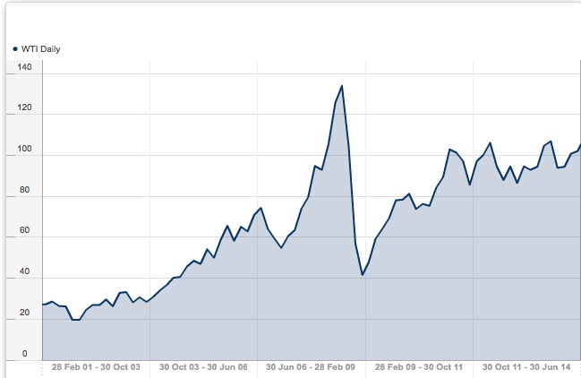
For free, historical data on commodities like Oil, you can try this site: http://www.databank.rbs.com This site will download data directly into spreadsheets for you, plot graphs of historical data, etc. Here is an example of oil prices (West Texas Intermdiate), over the last 15 years. Look how low it goes...
Yahoo supplies current stock and commodity prices. Here is an intereting site that tells you how to download loads of data into a csv file. http://www.financialwisdomforum.org/gummy-stuff/Yahoo-data.htm
Here is another site that discusses accessing various financial data sources. http://quant.stackexchange.com/questions/141/what-data-sources-are-available-online
Loading data off the web
To get away from the highly contentious issues of oil prices and political parties, let's look at some simple stock prices -- say Apple and Microsoft. We can import some basic webtools to get prices directly from Yahoo.
# Get some basic tools
%pylab inline
from pandas import Series, DataFrame
import pandas as pd
import pandas.io.data as web
Populating the interactive namespace from numpy and matplotlib


/opt/conda/envs/python2/lib/python2.7/site-packages/pandas/io/data.py:35: FutureWarning:
The pandas.io.data module is moved to a separate package (pandas-datareader) and will be removed from pandas in a future version.
After installing the pandas-datareader package (https://github.com/pydata/pandas-datareader), you can change the import ``from pandas.io import data, wb`` to ``from pandas_datareader import data, wb``.
  FutureWarning)
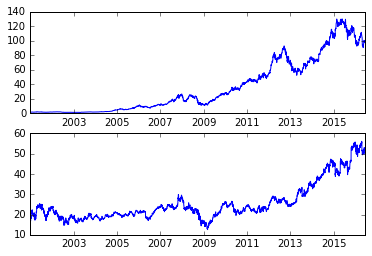
# Here are apple and microsoft closing prices since 2001
aapl = web.get_data_yahoo('AAPL','2001-01-01')['Adj Close']
msft = web.get_data_yahoo('MSFT','2001-01-01')['Adj Close']
subplot(2,1,1)
plot(aapl)
subplot(2,1,2)
plot(msft)
[<matplotlib.lines.Line2D at 0x7fa262183a90>]
aapl
Date
2001-01-02      0.978015
2001-01-03      1.076639
2001-01-04      1.121841
2001-01-05      1.076639
2001-01-08      1.088967
2001-01-09      1.130060
2001-01-10      1.088967
2001-01-11      1.183481
2001-01-12      1.130060
2001-01-16      1.125950
2001-01-17      1.105404
2001-01-18      1.228683
2001-01-19      1.282104
2001-01-22      1.265667
2001-01-23      1.347853
2001-01-24      1.347853
2001-01-25      1.310869
2001-01-26      1.286213
2001-01-29      1.425930
2001-01-30      1.430039
2001-01-31      1.421820
2001-02-01      1.388946
2001-02-02      1.356072
2001-02-05      1.327306
2001-02-06      1.388946
2001-02-07      1.364290
2001-02-08      1.364290
2001-02-09      1.257448
2001-02-12      1.294432
2001-02-13      1.257448
                 ...
2016-05-04     93.620002
2016-05-05     93.239998
2016-05-06     92.720001
2016-05-09     92.790001
2016-05-10     93.419998
2016-05-11     92.510002
2016-05-12     90.339996
2016-05-13     90.519997
2016-05-16     93.879997
2016-05-17     93.489998
2016-05-18     94.559998
2016-05-19     94.199997
2016-05-20     95.220001
2016-05-23     96.430000
2016-05-24     97.900002
2016-05-25     99.620003
2016-05-26    100.410004
2016-05-27    100.349998
2016-05-31     99.860001
2016-06-01     98.459999
2016-06-02     97.720001
2016-06-03     97.919998
2016-06-06     98.629997
2016-06-07     99.029999
2016-06-08     98.940002
2016-06-09     99.650002
2016-06-10     98.830002
2016-06-13     97.339996
2016-06-14     97.459999
2016-06-15     97.139999
Name: Adj Close, dtype: float64
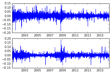
# Let's look at the changes in the stock prices, normalized as a percentage
aapl_rets = aapl.pct_change()
msft_rets = msft.pct_change()
subplot(2,1,1)
plot(aapl_rets)
subplot(2,1,2)
plot(msft_rets)
[<matplotlib.lines.Line2D at 0x7fa2617a5990>]
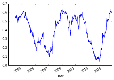
# Let's look at the correlation between these two series
pd.rolling_corr(aapl_rets, msft_rets, 250).plot()
/opt/conda/envs/python2/lib/python2.7/site-packages/ipykernel/__main__.py:2: FutureWarning: pd.rolling_corr is deprecated for Series and will be removed in a future version, replace with
    Series.rolling(window=250).corr(other=<Series>)
  from ipykernel import kernelapp as app


<matplotlib.axes._subplots.AxesSubplot at 0x7fa262d44a10>
Getting fancy.
Now, we can use some more sophisticated statistical tools, like least squares regression. However, I had to do some work to get Python to recognize these items. But I didn't work too hard, I just followed the error messages.
It became clear that I needed to go back to a terminal window to load in some packages. The two commands I had to type in were
- pip install statsmodels
- pip install patsy
'pip' is an 'python installer package' that install packages of code onto your computer (or whatever machine is running your python). The two packages 'statsmodels' and 'patsy' are assorted statistical packages. I don't know much about them, but they are easy to find on the web.
# We may also try a least square regression, also built in as a panda function
model = pd.ols(y=aapl_rets, x={'MSFT': msft_rets},window=256)
/opt/conda/envs/python2/lib/python2.7/site-packages/ipykernel/__main__.py:2: FutureWarning: The pandas.stats.ols module is deprecated and will be removed in a future version. We refer to external packages like statsmodels, see some examples here: http://statsmodels.sourceforge.net/stable/regression.html
  from ipykernel import kernelapp as app
model.beta
| MSFT | intercept | |
|---|---|---|
| Date | ||
| 2002-01-14 | 0.796463 | 0.000416 |
| 2002-01-15 | 0.788022 | 0.000417 |
| 2002-01-16 | 0.789784 | 0.000191 |
| 2002-01-17 | 0.802081 | 0.000600 |
| 2002-01-18 | 0.793941 | 0.000671 |
| 2002-01-22 | 0.796478 | 0.000718 |
| 2002-01-23 | 0.797909 | 0.001172 |
| 2002-01-24 | 0.786143 | 0.000960 |
| 2002-01-25 | 0.781526 | 0.001102 |
| 2002-01-28 | 0.782449 | 0.001064 |
| 2002-01-29 | 0.782113 | 0.001196 |
| 2002-01-30 | 0.764488 | 0.001069 |
| 2002-01-31 | 0.784935 | 0.001246 |
| 2002-02-01 | 0.784775 | 0.001254 |
| 2002-02-04 | 0.774178 | 0.001252 |
| 2002-02-05 | 0.781460 | 0.001383 |
| 2002-02-06 | 0.781529 | 0.001354 |
| 2002-02-07 | 0.792091 | 0.001506 |
| 2002-02-08 | 0.785451 | 0.001019 |
| 2002-02-11 | 0.788570 | 0.001084 |
| 2002-02-12 | 0.793316 | 0.001001 |
| 2002-02-13 | 0.796715 | 0.001117 |
| 2002-02-14 | 0.796227 | 0.001075 |
| 2002-02-15 | 0.801823 | 0.001176 |
| 2002-02-19 | 0.804453 | 0.000885 |
| 2002-02-20 | 0.814666 | 0.001097 |
| 2002-02-21 | 0.830058 | 0.000799 |
| 2002-02-22 | 0.818041 | 0.001174 |
| 2002-02-25 | 0.822848 | 0.001161 |
| 2002-02-26 | 0.821503 | 0.001248 |
| ... | ... | ... |
| 2016-05-04 | 0.634886 | -0.001187 |
| 2016-05-05 | 0.632351 | -0.001121 |
| 2016-05-06 | 0.631153 | -0.001282 |
| 2016-05-09 | 0.631186 | -0.001277 |
| 2016-05-10 | 0.627805 | -0.001240 |
| 2016-05-11 | 0.632612 | -0.001326 |
| 2016-05-12 | 0.629215 | -0.001440 |
| 2016-05-13 | 0.626302 | -0.001429 |
| 2016-05-16 | 0.631538 | -0.001302 |
| 2016-05-17 | 0.629171 | -0.001258 |
| 2016-05-18 | 0.629934 | -0.001218 |
| 2016-05-19 | 0.626321 | -0.001243 |
| 2016-05-20 | 0.627607 | -0.001232 |
| 2016-05-23 | 0.625496 | -0.001210 |
| 2016-05-24 | 0.624308 | -0.001229 |
| 2016-05-25 | 0.625938 | -0.001186 |
| 2016-05-26 | 0.625857 | -0.001192 |
| 2016-05-27 | 0.628037 | -0.001277 |
| 2016-05-31 | 0.624431 | -0.001256 |
| 2016-06-01 | 0.623145 | -0.001322 |
| 2016-06-02 | 0.623414 | -0.001335 |
| 2016-06-03 | 0.620833 | -0.001279 |
| 2016-06-06 | 0.621354 | -0.001256 |
| 2016-06-07 | 0.621346 | -0.001237 |
| 2016-06-08 | 0.621420 | -0.001246 |
| 2016-06-09 | 0.620108 | -0.001200 |
| 2016-06-10 | 0.620255 | -0.001216 |
| 2016-06-13 | 0.619448 | -0.001207 |
| 2016-06-14 | 0.618853 | -0.001180 |
| 2016-06-15 | 0.618974 | -0.001180 |
3631 rows × 2 columns
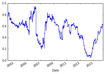
model.beta['MSFT'].plot()
<matplotlib.axes._subplots.AxesSubplot at 0x7fa2617a5550>
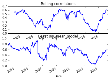
# Those two graphs looked similar. Let's plot them together
subplot(2,1,1)
pd.rolling_corr(aapl_rets, msft_rets, 250).plot()
title('Rolling correlations')
subplot(2,1,2)
model.beta['MSFT'].plot()
title('Least squaresn model')
/opt/conda/envs/python2/lib/python2.7/site-packages/ipykernel/__main__.py:3: FutureWarning: pd.rolling_corr is deprecated for Series and will be removed in a future version, replace with
    Series.rolling(window=250).corr(other=<Series>)
  app.launch_new_instance()


<matplotlib.text.Text at 0x7fa24cf18d90>
more stocks
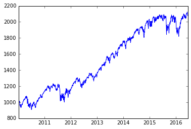
There is all kinds of neat info on the web. Here is the SPY exchange-traded fund, which tracks the S&P 500 index.
px = web.get_data_yahoo('SPY')['Adj Close']*10
px
Date
2010-01-04     998.08658
2010-01-05    1000.72861
2010-01-06    1001.43318
2010-01-07    1005.66052
2010-01-08    1009.00712
2010-01-11    1010.41626
2010-01-12    1000.99287
2010-01-13    1009.44749
2010-01-14    1012.17761
2010-01-15    1000.81670
2010-01-19    1013.32249
2010-01-20    1003.01842
2010-01-21     983.73128
2010-01-22     961.80210
2010-01-25     966.73395
2010-01-26     962.68278
2010-01-27     967.26241
2010-01-28     956.16569
2010-01-29     945.77354
2010-02-01     960.48105
2010-02-02     972.10617
2010-02-03     967.26241
2010-02-04     937.40701
2010-02-05     939.34454
2010-02-08     932.56318
2010-02-09     944.27638
2010-02-10     942.42694
2010-02-11     952.29063
2010-02-12     951.49804
2010-02-16     966.46975
                 ...
2016-05-04    2050.09995
2016-05-05    2049.70001
2016-05-06    2057.20001
2016-05-09    2058.89999
2016-05-10    2084.49997
2016-05-11    2065.00000
2016-05-12    2065.59998
2016-05-13    2047.59995
2016-05-16    2067.79999
2016-05-17    2048.50006
2016-05-18    2049.10004
2016-05-19    2041.99997
2016-05-20    2054.90005
2016-05-23    2052.10007
2016-05-24    2078.69995
2016-05-25    2092.79999
2016-05-26    2093.39996
2016-05-27    2102.40005
2016-05-31    2098.39996
2016-06-01    2102.70004
2016-06-02    2109.10004
2016-06-03    2102.79999
2016-06-06    2113.50006
2016-06-07    2116.79993
2016-06-08    2123.69995
2016-06-09    2120.80002
2016-06-10    2100.70007
2016-06-13    2084.49997
2016-06-14    2080.39993
2016-06-15    2077.50000
Name: Adj Close, dtype: float64
plot(px)
[<matplotlib.lines.Line2D at 0x7fa24ce5fa90>]